Your model is already outdated: online Machine Learning training with Apache Kafka and DJL

Machine Learning (ML) has transformed how we build intelligent systems, from recommendation engines to fraud detection. But most ML workflows still follow a pattern rooted in the batch processing era: collect a large dataset, train a model offline, deploy it, and retrain periodically when performance degrades. This works well when data is static and the world doesn’t change too fast. But what happens when your data arrives continuously, patterns shift in real time, and stale models cost you money or trust?

This is where data streaming meets machine learning, and where the real opportunity lies for data engineers already building event-driven architectures.

Why streaming data matters for Machine Learning

Traditional ML pipelines treat training as a one-time (or periodic) batch job. You gather historical data, train a model for hours or days, validate it, and push it to production. Days or weeks later, you repeat the cycle. The model is always learning from the past, never the present.

For many real-world applications, this lag is a problem. Consider fraud detection, where new attack patterns emerge daily, or IoT monitoring, where sensor readings can shift over time. A model trained last week may already be outdated. The faster your data moves, the faster your model should learn.

This is the problem known as model drift. The real-world patterns that a model learned during training gradually change, but the model itself stays frozen. Over time, the gap between what the model expects and what actually happens widens, and inference accuracy degrades. The model isn’t broken; the world has simply moved on. The only way to keep up is to keep learning.

Data streaming platforms like Apache Kafka have already solved the “how do we move data in real time” problem for application architectures. The natural next step is to ask: can we also train our models in real time, directly on the same streaming data?

The answer is yes, through a paradigm called online learning.

Online learning: training without stopping

In traditional (batch) Machine Learning, the model sees the entire dataset multiple times during training. Each full pass through the dataset is called an epoch, and training typically requires many epochs before the model converges.

Online learning flips this approach. Instead of iterating over a fixed dataset, the model processes data as it arrives, one batch at a time, learning incrementally and never looking back. There is no concept of epochs. Each batch of data contributes to the model’s knowledge and is then discarded.

This approach has several practical benefits:

• No need for large, pre-collected datasets. The model starts learning from the first batch of data.
• Adapts to changing patterns. Since the model continuously updates, it naturally adjusts to concept drift (when the statistical properties of the data change over time).
• Lower resource requirements. You don’t need to store and reprocess massive historical datasets. The model trains on small batches in memory.
• Continuous improvement. Rather than periodic retraining cycles, the model gets better over time as it sees more data.

The tradeoff is that online learning requires careful design. The model must be stable enough to learn meaningful patterns from small batches without forgetting what it learned earlier, and you need a way to evaluate whether the model is actually improving.

Deep Java Library: deep learning for Java developers

If you work in the Java ecosystem, you might assume that deep learning requires switching to Python. The Deep Java Library (DJL) challenges that assumption. DJL is an open-source framework, created and led by AWS, that brings deep learning to Java with an idiomatic, developer-friendly API. It is licensed under Apache 2.0 and the source code is available on GitHub.

DJL’s key design principle is engine abstraction. Rather than tying you to a single deep learning framework, DJL provides a unified API that works across multiple backends including PyTorch, TensorFlow, Apache MXNet, and ONNX Runtime. You can switch engines by swapping a Maven dependency, with no code changes required. Under the hood, your models still run on the same native engines used in the Python world, so there is no compromise on performance or accuracy.

For Java developers, DJL provides the building blocks you need for the full ML lifecycle:

• NDArray, a NumPy-like tensor abstraction for Java that serves as the foundation for all data operations.
• A neural network API with composable blocks for building architectures, from simple linear layers to multi-layer perceptrons and beyond.
• A training API with built-in support for optimizers (like Adam and SGD), loss functions, evaluators, and training listeners.
• An inference API with translators that handle the pre and post-processing between your Java objects and the tensors the model expects.
• A Model Zoo that provides pre-trained models for common tasks across computer vision, natural language processing, and more, ready to use out of the box.

For this demo, DJL is what makes it possible to build a complete online training and inference system entirely in Java, using the same build tools, IDE, and deployment patterns that Java developers already know.

Online training and inference in action with Apache Kafka and DJL

To explore these ideas in practice, I built a demo application that combines online Machine Learning training with Apache Kafka as the streaming data transport, and DJL with a PyTorch backend for the Machine Learning layer. This keeps the entire stack in the Java ecosystem.

The full source code is available on GitHub at github.com/ppatierno/ai-ml-streaming, including step-by-step instructions in the README for setting up Kafka, producing synthetic data, and running the training and inference pipelines.

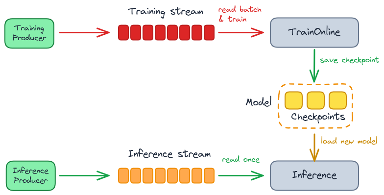
The system has two independent components: a training pipeline and an inference pipeline, connected only through model checkpoints on the filesystem.

How the training pipeline works

The demo uses synthetic data that simulates a 10-class classification problem. Each sample consists of a 784-dimensional feature vector (representing a flattened 28x28 image) and a class label (0 through 9). A Kafka producer generates these training samples and publishes them to a training-data topic.

The training application is a Kafka consumer that subscribes to this topic. As messages arrive, they are accumulated into batches. Each batch is fed directly into the model for a single training step. A forward pass computes predictions, the loss function measures how wrong those predictions are, backpropagation computes gradients, and the optimizer updates the model weights. Then the batch is discarded and the next one is processed.

Every 20 batches, the training application saves a checkpoint of the current model state to disk. These checkpoints are the bridge between training and inference.

How the inference pipeline works

The inference application runs as a separate process. It monitors the checkpoint directory, polling every few seconds for new or updated model files. When it detects a fresh checkpoint, it loads the updated model and runs predictions on a fixed set of evaluation samples.

By using the same evaluation set every time, the inference pipeline tracks accuracy across successive checkpoints, showing in real time whether the model is actually improving as it consumes more training data. You can watch the accuracy climb from near-random in the early batches to increasingly accurate predictions as the model converges.

Architecture at a glance

The training and inference pipelines are fully decoupled. The training application doesn’t know or care about inference; it just writes checkpoints. The inference application doesn’t know about training; it just watches for new model files. This separation makes each component independently scalable and replaceable.

Let’s walk through the key stages of the pipeline with short code excerpts from the demo.

Producing training data to Kafka

The pipeline starts with a Kafka producer that generates training samples and publishes them to the training-data topic. Each message is a JSON object carrying the feature vector and class label:

TrainingSample sample = generateSample();
String json = sampleToJson(sample);

ProducerRecord<String, String> record = new ProducerRecord<>(topic, json);
producer.send(record);

A separate producer does the same for the inference-data topic, generating a fixed evaluation set that will be used later to measure model accuracy.

Consuming and batching data from Kafka

On the training side, a Kafka consumer subscribes to the training-data topic and accumulates messages into batches. The KafkaDataSource class implements a DataSource interface that abstracts this away behind a simple nextBatch() call, which uses DJL’s NDArray API to convert the raw float arrays from each JSON message into the multidimensional tensors the model expects:

while (samples.size() < batchSize) {
    ConsumerRecords<String, String> records = consumer.poll(pollTimeout);
    for (ConsumerRecord<String, String> record : records) {
        TrainingSample sample = parseSample(record.value());
        samples.add(sample);
    }
}
return createBatch(manager, samples);

The training loop doesn’t know whether data comes from Kafka or a synthetic generator. It just calls nextBatch() and gets a ready-to-use DJL Batch object.

Configuring the model and trainer with DJL

With DJL, setting up the model and trainer is straightforward. We define a multi-layer perceptron using the ready-made Mlp block from DJL’s neural network API, with an input layer matching our 784-dimensional features, two hidden layers, and an output layer for the 10 classes. The training configuration uses DJL’s training API to wire together the loss function (softmax cross-entropy), an accuracy evaluator, and the Adam optimizer:

Model model = Model.newInstance("online-mlp");
Block block = new Mlp(INPUT_SIZE, NUM_CLASSES, new int[]{128, 64});
model.setBlock(block);

DefaultTrainingConfig config =
        new DefaultTrainingConfig(Loss.softmaxCrossEntropyLoss())
                .addEvaluator(new Accuracy())
                .addTrainingListeners(TrainingListener.Defaults.logging());

Trainer trainer = model.newTrainer(config);
trainer.initialize(new Shape(1, INPUT_SIZE));

Learning batch by batch from the stream

This is where online learning diverges from traditional training. There is no epoch loop. Instead, a single continuous loop processes batches as they arrive from the stream. Each batch goes through one training step: forward pass, loss computation, backpropagation, and weight update. Then the batch is discarded:

while (dataStream.hasNext()) {
    try (Batch batch = dataStream.nextBatch(trainer.getManager())) {
        EasyTrain.trainBatch(trainer, batch);
        trainer.step();
    }
}

The model learns incrementally, one batch at a time, never revisiting old data.

As the training process runs, you can observe the model learning in real time through the application logs. The accuracy starts low, as the model is essentially guessing, and steadily climbs as more batches are processed. In the example below, accuracy rises from 29% after 60 batches to 70% after 210 batches, while the loss decreases accordingly.

Training:      6% |███                                     | Accuracy: 0.29, SoftmaxCrossEntropyLoss: 2.11, speed: 87.12 items/sec14:14:08.289 [io.ppatierno.onlinetraining.training.TrainOnlineWithStreamingData.main()] INFO  io.ppatierno.onlinetraining.training.TrainOnlineWithStreamingData - Batch 60: Processed 1920 samples total
14:14:08.290 [io.ppatierno.onlinetraining.training.TrainOnlineWithStreamingData.main()] INFO  io.ppatierno.onlinetraining.training.TrainOnlineWithStreamingData - Checkpoint saved at batch 60 (1920 samples)
...
...
Training:     21% |█████████                               | Accuracy: 0.70, SoftmaxCrossEntropyLoss: 1.22, speed: 92.23 items/sec14:15:01.500 [io.ppatierno.onlinetraining.training.TrainOnlineWithStreamingData.main()] INFO  io.ppatierno.onlinetraining.training.TrainOnlineWithStreamingData - Batch 210: Processed 6720 samples total

Checkpointing: saving and resuming model state

Every 20 batches, the training application saves a snapshot of the model to disk. These checkpoints include metadata about how much data the model has seen, creating a trail of the model’s evolution:

if (batchCount % CHECKPOINT_FREQUENCY == 0) {
    model.setProperty("BatchCount", String.valueOf(batchCount));
    model.setProperty("TotalSamples", String.valueOf(totalSamples));
    model.save(checkpointDir, "online-mlp");
}

Checkpoints serve a dual purpose. They are the bridge between training and inference, and they also enable training resumption. When the training application starts, it checks for existing checkpoints and loads the most recent one before processing new data:

if (Files.exists(checkpointDir)) {
    try {
        model.load(checkpointDir, "online-mlp");
        logger.info("Resumed training from checkpoint");
    } catch (Exception e) {
        logger.info("No valid checkpoint found, starting fresh");
    }
}

This means the training process can be stopped and restarted without losing progress, an important property for any long-running streaming application. If the consumer crashes or needs to be redeployed, it picks up the model state from the last checkpoint and continues learning from where it left off.

Evaluating accuracy with live model updates

The inference application runs as a separate process. When it detects a new checkpoint, it loads the model and uses DJL’s inference API to evaluate accuracy against the fixed set of samples consumed from the inference-data Kafka topic. A Predictor with a NoopTranslator runs predictions directly at the NDArray level, bypassing any pre/post-processing since the data is already in tensor-ready form:

Model model = Model.newInstance("online-mlp");
model.setBlock(new Mlp(INPUT_SIZE, NUM_CLASSES, new int[]{128, 64}));
model.load(checkpointDir, "online-mlp");

try (Predictor<NDList, NDList> predictor =
        model.newPredictor(new NoopTranslator())) {
    for (InferenceSample sample : inferenceSet) {
        NDList input = new NDList(manager.create(sample.features));
        NDList result = predictor.predict(input);
        long predicted = result.singletonOrThrow().argMax().getLong();
    }
}

By using the same evaluation set every time, the inference pipeline tracks how accuracy improves across successive checkpoints, from near-random early on to increasingly accurate predictions as the model converges.

As the inference process picks up new checkpoints, you can see the accuracy improve in real time. In the example below, the model starts at 36% accuracy after just 40 batches of training, and reaches nearly 98% after 160 batches, all without restarting the inference application.

14:14:03.531 [io.ppatierno.onlinetraining.inference.InferenceWithStreamingCheckpoints.main()] INFO  io.ppatierno.onlinetraining.inference.InferenceWithStreamingCheckpoints -   Training Progress: 40 batches, 1280 samples
Inference:   100% |████████████████████████████████████████|
14:14:03.876 [io.ppatierno.onlinetraining.inference.InferenceWithStreamingCheckpoints.main()] INFO  io.ppatierno.onlinetraining.inference.InferenceWithStreamingCheckpoints -   Inference Accuracy: 363/1000 (36.30%)
...
...
14:14:44.850 [io.ppatierno.onlinetraining.inference.InferenceWithStreamingCheckpoints.main()] INFO  io.ppatierno.onlinetraining.inference.InferenceWithStreamingCheckpoints -   Training Progress: 160 batches, 5120 samples
Inference:   100% |████████████████████████████████████████|
14:14:44.974 [io.ppatierno.onlinetraining.inference.InferenceWithStreamingCheckpoints.main()] INFO  io.ppatierno.onlinetraining.inference.InferenceWithStreamingCheckpoints -   Inference Accuracy: 978/1000 (97.80%)

Optimizer choice: Adam vs. Passive-Aggressive

The demo supports two different optimizer and model architecture combinations. The first uses Adam, a widely adopted optimizer, paired with a multi-layer perceptron (MLP) neural network. This is a solid general-purpose choice that works well across a range of problems.

The second option uses the Passive-Aggressive algorithm, an optimizer specifically designed for online learning scenarios. It pairs with a simpler linear model. The Passive-Aggressive algorithm gets its name from its behavior: it is passive when a prediction is correct (making no update to the model), and aggressive when a prediction is wrong (making the minimum update needed to correct the error). This makes it particularly efficient for streaming scenarios where you want fast, meaningful updates from each batch.

Both approaches achieve strong accuracy on the demo’s classification task, but they represent different philosophies. Adam and the MLP offer more modeling capacity and flexibility, while Passive-Aggressive with a linear model is purpose-built for the online learning paradigm.

What this means for data engineers

If you’re already building event-driven systems with Kafka, adding online ML training to your architecture doesn’t require a paradigm shift. The training application is just another Kafka consumer. The inference application is just another service that reacts to state changes (in this case, new model files). The patterns are familiar: producers publish data, consumers process it, and the system’s components communicate through well-defined interfaces rather than tight coupling.

Look at the architecture through the lens of what you already build daily. The training consumer uses consumer groups, so you can scale it horizontally or restart it without losing your position in the topic. Checkpoints are the model’s equivalent of a stateful store: they capture the learned state so it survives restarts and can be picked up by a completely separate process. The training and inference pipelines are decoupled the same way any two Kafka-based services are, through a shared contract (the checkpoint format) rather than direct calls.

This demo is intentionally simple, using synthetic data and a straightforward classification task. But the architecture points toward concrete next steps:

• Use real event streams. Replace the synthetic producer with a connector or application that publishes actual user interactions, sensor readings, or transaction events. The training consumer doesn’t care where the data comes from as long as the message format matches.
• Add schema validation. In a production pipeline, you would register the training sample schema in a Schema Registry and use Avro or Protobuf serialization instead of plain JSON, giving you backward compatibility guarantees as the feature set evolves.
• Externalize the model store. The demo writes checkpoints to the local filesystem. Moving them to an object store like S3 or MinIO lets the inference service run on a different machine and opens the door to versioned model management.
• Monitor model quality as a metric. Treat inference accuracy the same way you treat consumer lag or throughput: publish it to your observability stack and alert when it degrades, because a drifting model is an operational problem, not just a data science one.

The gap between data engineering and machine learning is narrower than it seems. The tools and patterns you already know are the same ones that power real-time ML.